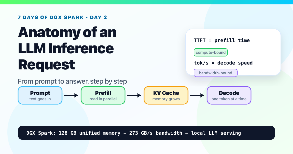
Day 2: Anatomy of an LLM Inference Request. From Prompt to Answer, Step by Step
A beginner-friendly walkthrough of tokenization, prefill, KV cache, decode, batching, TTFT, and why memory bandwidth shapes local LLM performance on NVIDIA DGX Spark.

New to the jargon? Every term, flag, and benchmark number here is explained in plain English in the local LLM glossary.
On this page (19)
- The whole lifecycle in one picture
- Step 1: Tokenization (text → integers)
- Step 2: Prefill (the model reads your prompt)
- What does "read" mean for a model?
- The good news: prefill is embarrassingly parallel
- A concrete walk-through: "What's the capital of France?"
- So what limits prefill speed?
- What that looks like on a real Spark
- So can you make prefill faster?
- Attention in plain English (the bridge to KV cache)
- Step 3: The KV cache (the magic that makes decode possible)
- So what happens when the cache fills the 128 GB?
- Step 4: Decode (the memory-bandwidth-bound phase)
- Why batching changes everything
- A short peek at what serving engines do on top
- Why "tok/s" is two numbers, not one
- Putting it together: a real request trace
- What this means for picking hardware
- What's coming on Day 3
Day 2 of "7 Days of Local LLM". A field guide to running serious LLMs on a $4,699 box on your desk.
On Day 1 you ran your first local LLM on the Spark. You typed something into Ollama and the model wrote back. Today we look at what's actually happening inside the box while that little back-and-forth is going on.
Let's make it concrete. Imagine you ask the local model:
You: What's the capital of France?
A few seconds later, the model writes back:
Model: Paris.
That's it. A question goes in, an answer comes out. From the outside it can look like one big magical step: the model "thought about it" and replied. But that's not what's happening inside the computer. Inside, the Spark is running a small assembly line of four phases, every single time:
- Read your question - turn your text into numbers the model can work with.
- Absorb the prompt - the model "looks at" your whole question in one go.
- Write the answer - the model generates its reply one piece at a time.
- Show you the answer - turn those pieces back into text on your screen.
That's the whole story at the high level. Four phases, in order. Think of that as the beginner map. In the lifecycle below, we'll split the same flow into six smaller systems steps so the performance pieces are easier to see.
Once you can see those phases as separate things, a lot of weird LLM behavior stops being weird. By the end of this post you'll understand:
- Why "tokens per second" is actually two different numbers, not one
- Why a 70-billion-parameter model on a Spark generates only about 7 tokens per second, even though the chip can do trillions of math operations per second
- Why serving 16 users at once can be surprisingly close to serving one, until the GPU saturates
- Why the same model on the same hardware can feel snappy for one prompt and sluggish for another
You don't need a computer-science background to follow along. Every term gets defined when it first shows up. Let's walk through the four phases.
The whole lifecycle in one picture #
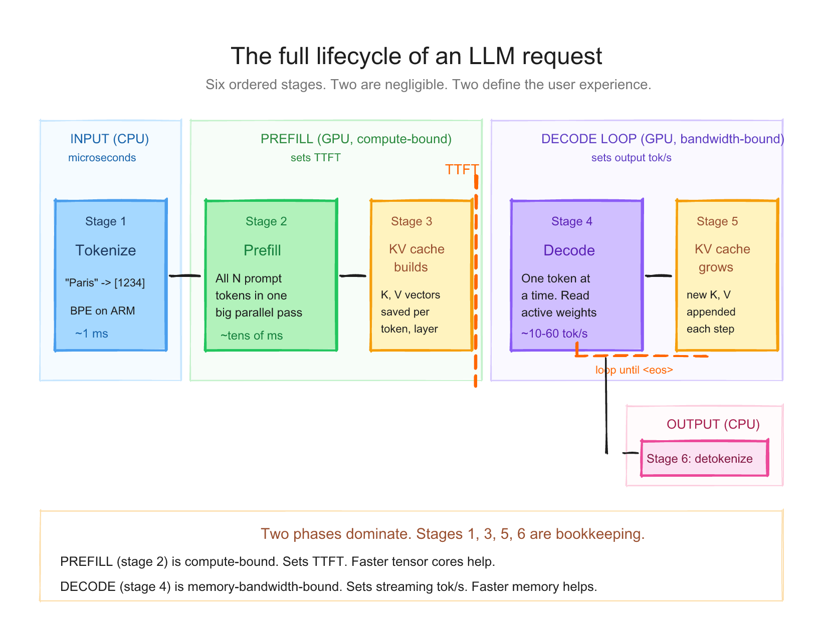
When you send a prompt to an LLM, six things happen in order. Each one is a distinct piece of work.
- Tokenization, your text becomes integers
- Prefill, the model reads the entire prompt at once
- KV cache builds up, the model remembers what it just read
- Decode, the model generates new tokens, one at a time
- KV cache grows, each new token gets added
- Detokenization, integers become text again
Steps 1 and 6 are negligible. Steps 2 and 4 are the whole game. Step 3 is the magic that makes step 4 possible.
Let me walk through each.
Animated Request Trace
From prompt to streamed answer
The request has two expensive phases: prefill reads the whole prompt in parallel, then decode loops one output token at a time while reusing the KV cache.
Step 1: Tokenization (text → integers) #
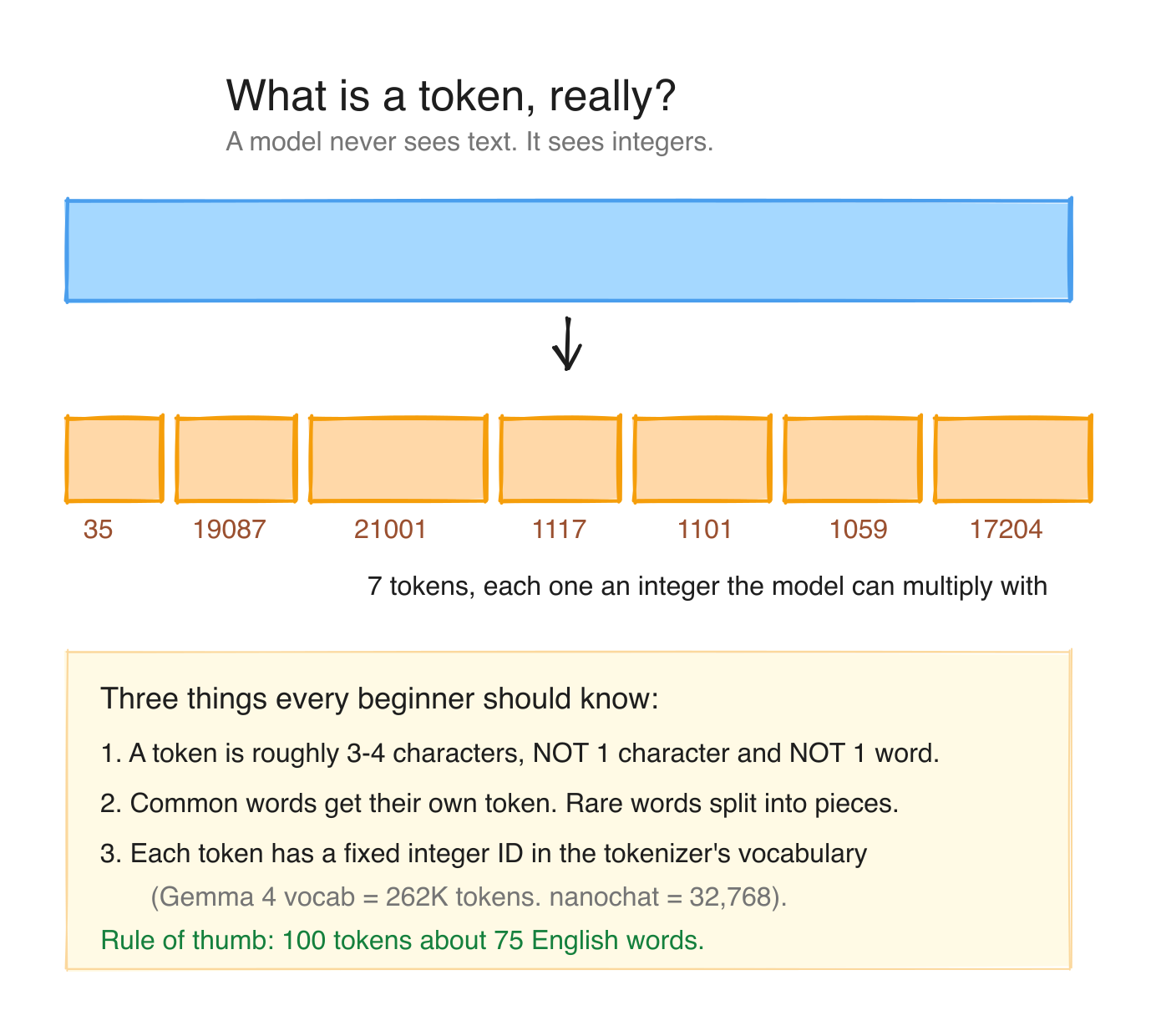
LLMs do not read characters. They read tokens. A token is an integer that maps to a piece of text. The mapping is fixed for a given model. It comes from training.
The most common tokenization scheme today is Byte Pair Encoding (BPE). The intuition: take the most frequently co-occurring pairs of characters in your training corpus, merge them into a single token, repeat. After a few thousand iterations, you have a vocabulary of ~30,000 to ~262,000 tokens, depending on the model family, where common words are usually one token, uncommon words are two or three tokens, and rare unicode is per-byte.
Quick examples (from a typical Llama-family tokenizer):
| Text | Tokens | Count |
|---|---|---|
"Paris" | ["Paris"] | 1 |
"capital" | ["capital"] | 1 |
"capitalism" | ["capital", "ism"] | 2 |
"What's the capital of France?" | ["What", "'s", " the", " capital", " of", " France", "?"] | 7 |
"スパーク" (Japanese "spark") | typically 3-6 byte tokens | 3-6 |
Two things to remember:
- Tokens are not words. A 100-word essay is usually 130-150 tokens.
- Tokenizer is per model family. Llama, Qwen, Gemma, Nemotron all have their own. Same text gives different token counts in different models.
Tokenization happens on the CPU and is essentially free. We're talking microseconds. It is not a bottleneck.
Step 2: Prefill (the model reads your prompt) #
After tokenization, your text is a list of integers. Now the model has to actually read it before it can answer. This reading step is called prefill.
What does "read" mean for a model? #
Reading, for an LLM, means: take each token, run it through every layer of the network, and build up an internal representation of what the prompt is "about." A typical 8B-class model has somewhere around 30 layers; a 70B model has 80. Every layer does the same kind of work: a chunk of matrix multiplication (the model's stored weights times your data), then a chunk of attention math (each token deciding which earlier tokens matter), then a non-linear squish, and on to the next layer.
By the time your prompt has been through every layer, the model has a rich internal state that represents "I've read this. I understand the context. I'm ready to start writing." Only then can it produce the first output token.
The good news: prefill is embarrassingly parallel #
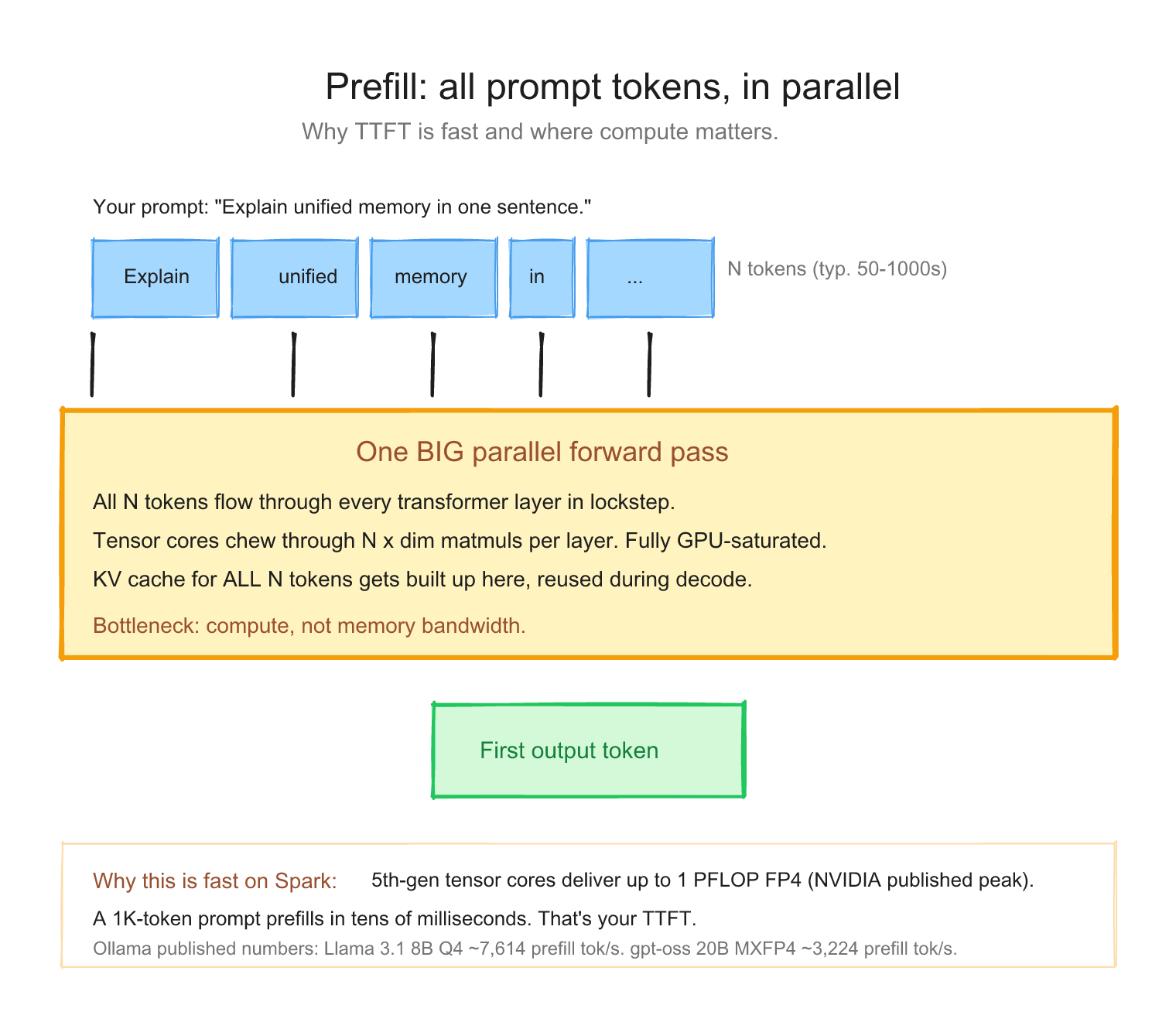
Here's the lucky bit. When the model reads your prompt, every token can be processed at the same time inside each layer.
Picture a 1,000-token prompt going through one layer. Instead of:
do token 1 → do token 2 → do token 3 → ... → do token 1000 (sequentially, slow)
the GPU does:
do all 1,000 tokens together as one giant matrix multiply (in parallel, fast)
This works because at layer N, each token only needs to "look at" tokens that came before it. Those values are all already known (they're your prompt; nothing is being generated yet). So the GPU can lay all 1,000 tokens side by side and crunch through them in one go.
That's what tensor cores are built for: enormous matrix multiplications. Prefill keeps them genuinely busy. This is why the prefill numbers in the Ollama benchmark look so big.
A concrete walk-through: "What's the capital of France?" #
Take our Paris example. After tokenization, you have 7 tokens: [What, 's, the, capital, of, France, ?]. You send those 7 tokens to a model with, say, 32 layers.
What the GPU does, layer by layer:
| Step | What's happening | Cost |
|---|---|---|
| Layer 1 | All 7 tokens go through one big matmul + attention together | one parallel pass |
| Layer 2 | Same again, but with layer 1's output as input | one parallel pass |
| ... | ... | ... |
| Layer 32 | Last pass, model now "understands" the prompt | one parallel pass |
So for 7 tokens × 32 layers, the GPU does 32 sequential layer passes, and each pass crunches all 7 tokens in one shot. For a tiny prompt like this, the 7-token width is almost free compared to the depth of 32 layer passes. (At long prompts, that stops being true: attention work in particular grows with the square of the sequence length, which is why a 50K-token RAG prompt takes meaningful prefill time.)
That's why even a 1,000-token prompt only takes hundreds of milliseconds to prefill on a Spark: the GPU is doing tens of thousands of tokens worth of math in parallel, all at once. Spreading the work across tokens is exactly what tensor cores are good at.
So what limits prefill speed? #
Two factors, in this order:
- The model. Bigger models (more layers, bigger hidden size) mean each layer pass is heavier, and there are more of them. A 70B model prefills slower per-token than an 8B model on the same hardware. That's not a surprise: there's literally more math to do.
- The hardware's raw math throughput. Tensor cores have a peak rate (in FLOPS, floating-point operations per second). The GB10 chip in Spark is rated for up to 1 PFLOP at FP4 sparse (NVIDIA's published peak). Whatever your model demands per token, the chip can only push so many FLOPS per second.
This is what "prefill is compute-bound" means: the bottleneck is the chip's math speed, not its memory speed. (Decode, the next step, is the opposite, and we'll see why in a minute.)
What that looks like on a real Spark #
Ollama's published Spark benchmark gives you concrete numbers:
| Model | Prefill rate |
|---|---|
| Llama 3.1 8B Q4 | ~7,614 tok/s |
| DeepSeek R1 14B Q4 | ~5,919 tok/s |
| GPT-OSS 20B MXFP4 | ~3,224 tok/s |
Read that table left to right and the story tells itself: bigger model = slower prefill on the same chip. Same GPU, same memory, the only thing that changed is how much math each token has to go through.
At those rates a 500-token prompt takes well under a second on the 8B model. By the time you hit enter, the model is already busy reading; by the time you blink, it's about to start writing.
So can you make prefill faster? #
Three knobs, in order of impact:
- Send fewer prompt tokens (no math, no time). RAG with 50K tokens of retrieved context will always be slower at TTFT than a 200-token chat turn, on the same model.
- Pick a smaller model if quality permits. A 4B model with a focused fine-tune often prefills 5-10x faster than a 70B and is good enough for the task.
- Batch multiple requests together so the GPU sees more work per pass. This is what serving engines like vLLM do automatically.
That's prefill. One big parallel chew through your prompt, limited by how fast the chip can do math. Up next: the cache that makes the writing phase possible.
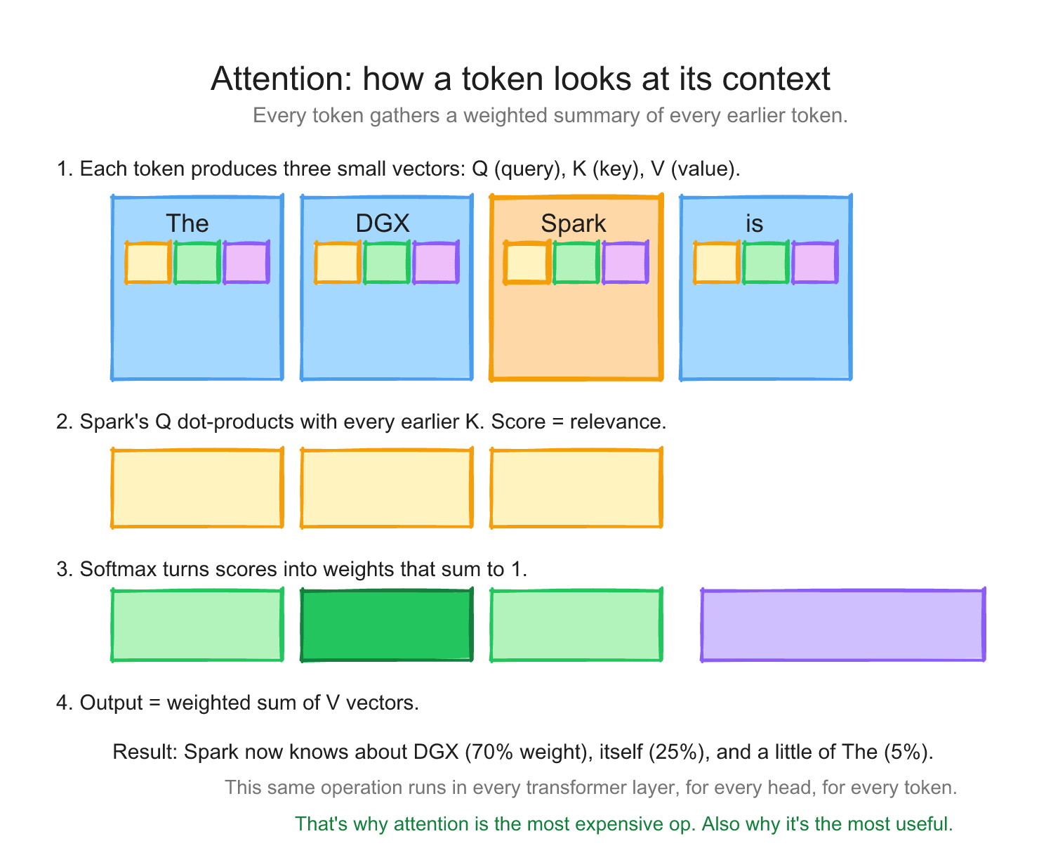
Attention in plain English (the bridge to KV cache) #
Before we talk about the KV cache, a one-paragraph mental model for what attention does.
For every token in your sequence, the model produces three vectors: a Query (Q), a Key (K), and a Value (V). Think of K as a "what I am" tag, V as the "what I contribute" payload, and Q as the "what I'm looking for" request. To decide how much each earlier token matters for the next prediction, the model compares the current Q against every previous K (a dot product), softmaxes those scores into weights, and uses them to blend the previous Vs. That blended vector goes into the next layer.
The important consequence for performance: once a token has produced its K and V, those vectors don't change. They only get looked at by every future token. Re-computing them on every decode step would be quadratically expensive and totally unnecessary. So we save them. That saved structure is the KV cache, and it's why decode can produce one token at a time without re-reading the whole conversation from scratch.
Step 3: The KV cache (the magic that makes decode possible) #
Here's where things get interesting. After prefill, the model has computed something called the key (K) and value (V) vectors for every token in your prompt, at every layer. These K and V vectors are what the model uses to do attention: "when I generate the next token, what previous tokens should I pay attention to?"
Naive question: when the model generates token 1001, does it have to re-process tokens 1 through 1000 again? Then for token 1002, re-process 1-1001? That would be quadratic and horrible.
The trick: cache the K and V vectors. Save them from prefill. For each new generated token, you only have to compute its own K and V, then attend to everything else from the cache.
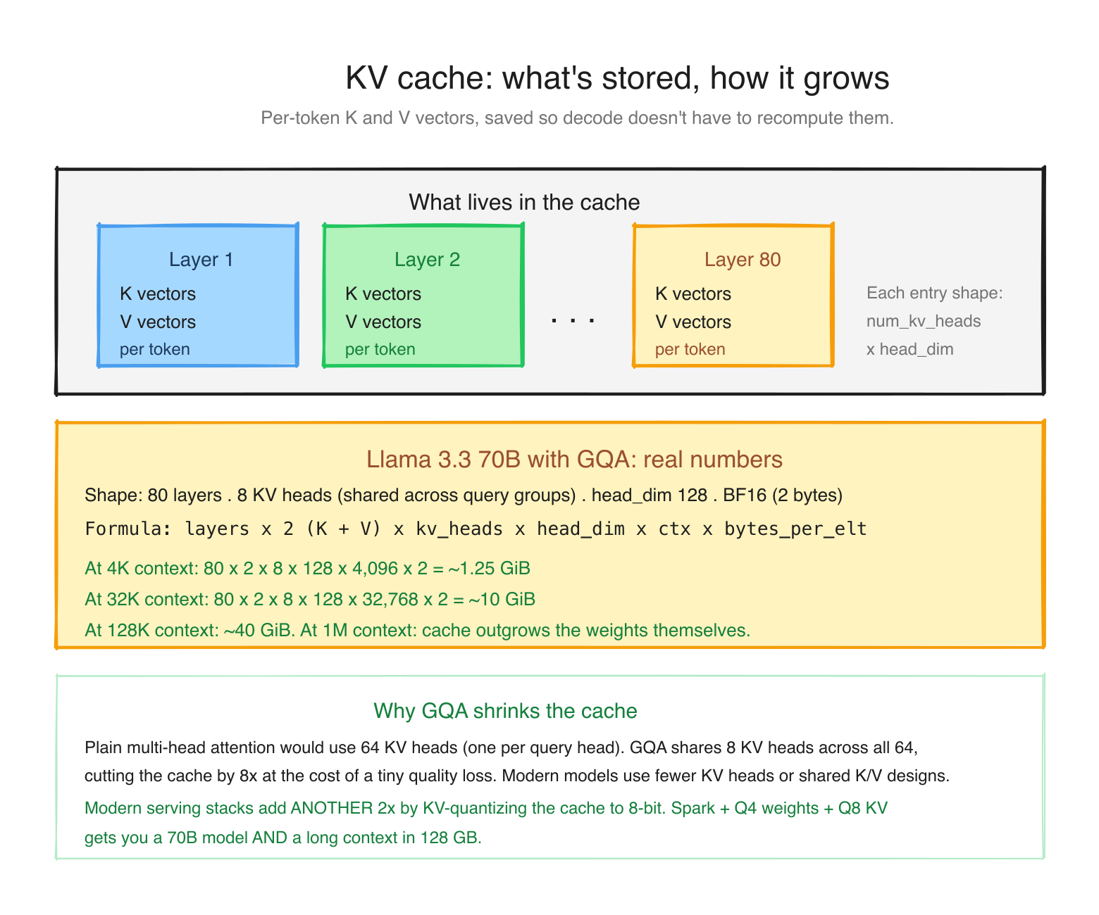
This cache is the KV cache. It grows as you generate. It is roughly:
KV cache size = num_layers × 2 (K and V) × num_kv_heads × head_dim × context_length × bytes_per_elementWhere does it live? This is where Spark differs from a normal PC.
- Regular machine (discrete GPU): the GPU has its own dedicated memory, called VRAM, physically separate from the computer's system RAM. That's 24 GB on an RTX 4090, 32 GB on a 5090, 80 GB on an H100. Both the model weights and the KV cache have to fit in that VRAM. Your system RAM might be much larger, but it sits on the other side of a slow PCIe link, so spilling the cache over there tanks performance.
- DGX Spark (unified memory): there is no separate GPU memory at all. The Grace CPU and the Blackwell GPU share one 128 GB LPDDR5x pool, and both see the same bytes with no copying. Model weights, KV cache, activations, and your OS all live together in that single pool.
So the question changes shape. On a regular machine you ask "does this fit in VRAM?" On a Spark you ask "does weights + KV cache + overhead fit in the one 128 GB pool?" Same budgeting problem, one pool instead of two. The mental model on Spark: the KV cache is just one more tenant competing for the same 128 GB as your model weights. (This is the unified-memory idea from Day 1; Day 3 opens it all the way up.)
One thing to be very clear about: bigger pool does not mean faster. A Spark having 128 GB while an H100 has 80 GB does not make the Spark a faster chip. The opposite, in fact. The two differ on three separate axes, and Spark only wins one of them:
| DGX Spark (GB10) | H100 (SXM, 80 GB) | |
|---|---|---|
| Memory capacity | 128 GB unified | 80 GB |
| Memory bandwidth | ~273 GB/s | ~3.35 TB/s (about 12x Spark) |
| GPU compute | 48 SMs, 6,144 CUDA cores, 5th-gen tensor cores | 132 SMs, ~16,896 CUDA cores |
| Price | ~$4,699 | ~$25,000-40,000 |
An H100 will decode the same model roughly an order of magnitude faster than a Spark, because decode speed tracks memory bandwidth (the next section is all about why), and the H100 has about 12x more of it. What the Spark gives you is capacity per dollar: it can hold a 70B or 120B model that does not fit in an H100's 80 GB at all, for a tenth of the price. You are not buying speed. You are buying "this large model runs on my desk at all."
And to answer the natural question, "if the memory is shared, how much actual GPU is in a Spark?" There is a real Blackwell GPU in there: 48 streaming multiprocessors, 6,144 CUDA cores, and 5th-generation tensor cores (the sm_121 part we keep mentioning). It is a genuine GPU. It simply reads from the shared 128 GB pool instead of from its own private VRAM. The compute is modest next to an H100's, but it is real GPU silicon, not a CPU pretending to be one. Day 3 takes the lid off all of it.
Modern 70B models like Llama 3.3 use Grouped-Query Attention (GQA), which shares K and V across multiple query heads to keep the cache small. Plugging Llama 3.3 70B's actual shape (80 layers, 8 KV heads, head_dim 128, BF16) into the formula: ~1.25 GiB at 4K context, ~10 GiB at 32K, ~40 GiB at 128K. At a million-token context the cache would be ~300 GB, which no single Spark can hold. This is why context length is expensive.
So what happens when the cache fills the 128 GB? #
This is the real constraint on Spark, and you asked exactly the right question. Add up your budget for a single request:
weights + KV cache + framework overhead + OS must fit in ~128 GB.
A Llama 3.3 70B at Q4 is ~40 GB of weights. Give it a 128K context and the KV cache is another ~40 GB. Add ~10 GB of OS and runtime overhead and you are at ~90 GB for one long-context request. Push the context further, or add concurrent users (each needs its own KV cache), and you hit the ceiling. When you cross it, the inference engine either refuses the request or, worse, slows to a crawl. You don't get a separate VRAM cliff like on a discrete GPU; you get one shared pool that you can overcommit.
Here is how people actually keep the cache under control, roughly in order of how often you'll reach for them:
- Quantize the KV cache. Store K and V in 8-bit (or even 4-bit) instead of 16-bit. That halves or quarters the cache for a small quality cost. In llama.cpp this is
--cache-type-k q8_0 --cache-type-v q8_0; vLLM and others have equivalents. This is the single biggest lever. - Cap the context window. If you do not need 128K tokens, do not allocate for it. Most engines let you set a max context (
--ctx-sizein llama.cpp,--max-model-lenin vLLM). Right-size it to your actual prompts. - Use PagedAttention. vLLM's KV cache manager treats the cache like virtual-memory pages, so you waste far less to fragmentation and pack more requests into the same pool. You don't tune anything; you just get more usable cache by choosing vLLM.
- Share prefixes. If many requests start with the same long system prompt or RAG bundle, compute that prefix's KV cache once and reuse it (SGLang's RadixAttention, vLLM's prefix caching). Huge win for agent and RAG workloads.
- Pick a smaller or sliding-window model. Some models (for example, Mistral-family) use sliding-window attention that only keeps the last N tokens' KV, so the cache stops growing past a fixed size.
We get into the engine-specific knobs on Day 5. For now the takeaway is: on Spark the KV cache and the weights live in the same 128 GB, and KV-quantization plus a sensible context cap is what keeps you off the cliff.
The KV cache is also why batching matters. The model's weights only need to be read from memory once per token, no matter how many concurrent requests are in flight. The KV cache, though, is per request. So if you have 16 requests in flight, you read the weights once and they "serve" all 16 KV caches in parallel, but you are also holding 16 KV caches in the pool at the same time. That's where the throughput multiplier comes from, and also why memory, not compute, is what caps your concurrency on Spark.
Step 4: Decode (the memory-bandwidth-bound phase) #
Now the model generates new tokens. One at a time. Each new token requires reading the entire model from memory, doing the matrix multiplications, looking at the KV cache for attention, and producing the next token.
Let's watch it happen on our example. After prefill, the model has read "What's the capital of France?" and its KV cache holds those 7 tokens. Now decode runs:
- Step 1: read the whole model from memory, look at the KV cache (7 prompt tokens), predict the next token:
Paris. Append it. Add its K and V to the cache (now 8 tokens). - Step 2: read the whole model again, look at the KV cache (8 tokens now), predict the next token: an end-of-sequence marker, the model's way of saying "I'm done."
- Stop.
So "Paris." cost two output tokens, two full reads of the model. If the answer had been 200 tokens long, that's 200 reads, strictly one after another, because each token can only be predicted once the previous one exists. That sequential, one-read-per-token rhythm is the entire reason decode is slow.
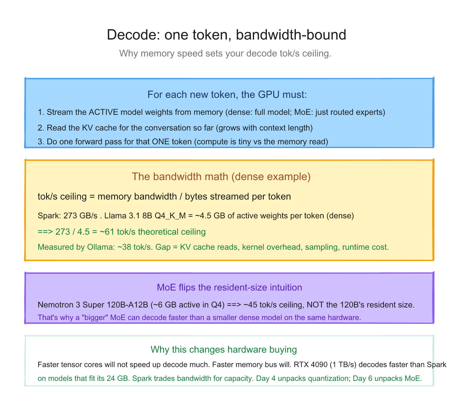
The crucial thing: for each generated token, roughly the active model weights have to be streamed from memory per output token. Every layer's weight matrix gets pulled into the tensor cores, multiplied against the activations, and (mostly) discarded. "Active" matters: for a dense model that's the whole model; for a Mixture-of-Experts model it's just the experts the router picks for that token.
The math: 273 GB/s memory bandwidth (Spark) divided by the bytes actually read per token equals your theoretical maximum tokens per second. For a dense model, "bytes read" = full model size. For an MoE, "bytes read" = active parameters × bytes/param, NOT the full resident model.
| Model | Resident size | Bytes read per token | Theoretical decode max | Type |
|---|---|---|---|---|
| Llama 3.1 8B Q4 | 4.5 GB | 4.5 GB (dense) | ~61 tok/s | dense |
| GPT-OSS 20B MXFP4 | 13 GB | ~3.6 GB (3.6B active params + shared attention layers) | ~75 tok/s | MoE |
| Llama 3.3 70B NVFP4 | 40 GB | 40 GB (dense) | ~6.8 tok/s | dense |
| Nemotron 3 Super 120B-A12B NVFP4 | 60 GB | ~6 GB (12B active) | ~45 tok/s | MoE |
This is why some "bigger" models decode faster than smaller dense ones: an MoE only reads its active parameters per token. Resident-size-based math is wrong for MoEs.
One important caveat: that last column is a ceiling, not a promise. It's the best you could ever do if memory bandwidth were the only cost. Real life is slower. On my own Spark, Nemotron 3 Super (Ollama Q4_K_M) measured 19.5 tok/s decode, well under the ~45 tok/s NVFP4 ceiling in the table. Three reasons for that specific gap: Q4_K_M is a heavier format than NVFP4 (more bytes per token), Nemotron 3 Super is a hybrid Mamba/MoE rather than a clean MoE so the active-parameter math is only an upper bound, and every token also pays for KV cache reads and kernel overhead. The ceiling tells you the shape of what to expect; the measured number tells you what you actually get.
Compare to published single-stream numbers from Ollama's official Spark benchmark: llama 3.1 8B at 38 tok/s, gpt-oss 20B at 58 tok/s, deepseek-r1 14B at 20 tok/s. Each sits below its theoretical ceiling for the same reasons. But the order of magnitude is set by memory bandwidth (and active-parameter count for MoEs), not by the GPU's compute power.
This is why decode is memory-bandwidth-bound, not compute-bound. The tensor cores spend most of their time waiting for weights to arrive from memory. Adding more tensor cores would not help. Adding more memory bandwidth would.
If you remember one number from this entire week, it's this: Spark's 273 GB/s memory bandwidth divided by your model's bytes in memory ≈ your decode tok/s.
Decode in plain words: the model writes the answer one token at a time. Each token is predicted from the KV cache (everything seen so far) plus one full read of the model's weights from memory. The tokens come out in sequence, each waiting for the last, until an end token appears. Because every token costs a trip to memory, decode speed is set by memory bandwidth, and decode is the part you feel as "typing speed" (tok/s).
Why batching changes everything #
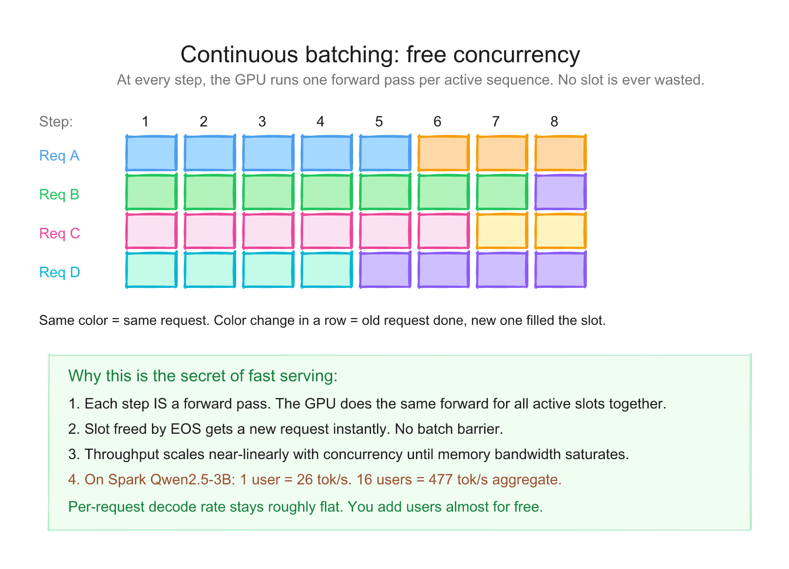
Here's the leverage. When you have one user generating one token, you read the entire model from memory to produce that token. One read, one token output.
When you have 16 users in flight, you read the entire model from memory to produce one token for each of them in the same pass. One read, 16 tokens output.
Animated Serving Model
Why batching changes the economics
One user makes the memory read expensive. Many users let one model read produce many output tokens in the same decode step.
The model read cost is amortized across all requests. Per-request latency stays roughly similar until you saturate the GPU. You can watch it drift down by a few percent as concurrency rises in the table below, then drop harder once you cross the saturation point. Aggregate throughput, meanwhile, climbs almost linearly until saturation.
I measured this directly on my DGX Spark. Gemma 4 31B IT in NVFP4, served via vLLM, max_tokens=512:
| Concurrent requests | Aggregate tok/s | Per-request tok/s |
|---|---|---|
| 1 | 6.15 | 6.15 |
| 4 | 24.41 | 6.10 |
| 8 | 47.13 | 5.89 |
| 16 | 92.10 | 5.76 |
| 32 | 166.36 | 5.20 |
Same model, same hardware, same prompt. Aggregate scales roughly linearly with concurrency while per-request latency stays inside a couple of tok/s. Same Spark same week, Qwen2.5-3B BF16: 26.14 → 125.72 → 246.79 → 476.95 → 851.84 → 1462.30 tok/s as N goes 1 → 4 → 8 → 16 → 32 → 64.
[An earlier 2026-05-08 capture of this same setup labeled c=4 numbers as c=8 (and so on, drifting one concurrency level too low). The 2026-05-21 numbers above are canonical for this series.]
Memory bandwidth amortization is the most important performance lever you have on Spark. Batch whenever your workload can tolerate it.
A short peek at what serving engines do on top #
Continuous batching is one of several tricks production serving engines use to stretch the same memory bandwidth further. Four other tricks are worth knowing by name, even if Day 2 doesn't deep-dive them:
- Prefill / decode disaggregation. Prefill is compute-bound and likes big batches; decode is bandwidth-bound and likes small responsive batches. Run them on separate GPU pools and hand off the KV cache between them, so one phase doesn't jitter the other. (Mostly an SGLang and TensorRT-LLM concern; covered briefly on Day 5.)
- Paged KV cache (PagedAttention). Instead of a contiguous KV block per request, treat the cache like virtual memory pages. Fragmentation drops, packing improves, larger effective batches fit. vLLM's original contribution; we open it up properly on Day 5.
- Prefix-aware routing. Don't round-robin requests blindly. If a new request shares a prefix (system prompt, RAG bundle) with a replica that already has that KV cache hot, route it there. SGLang's RadixAttention is the cleanest implementation; also on Day 5.
- MoE sharding and routing. Mixture-of-Experts models keep attention layers replicated and shard experts across devices. A token activates a small subset of experts. Day 6 covers what that means for picking a Spark-friendly model; Day 4 covers the format math.
For a single user on a single Spark, continuous batching alone gives you most of the win. The others matter when you're running multi-tenant serving, very long contexts, or MoE models that exceed a single device.
Why "tok/s" is two numbers, not one #
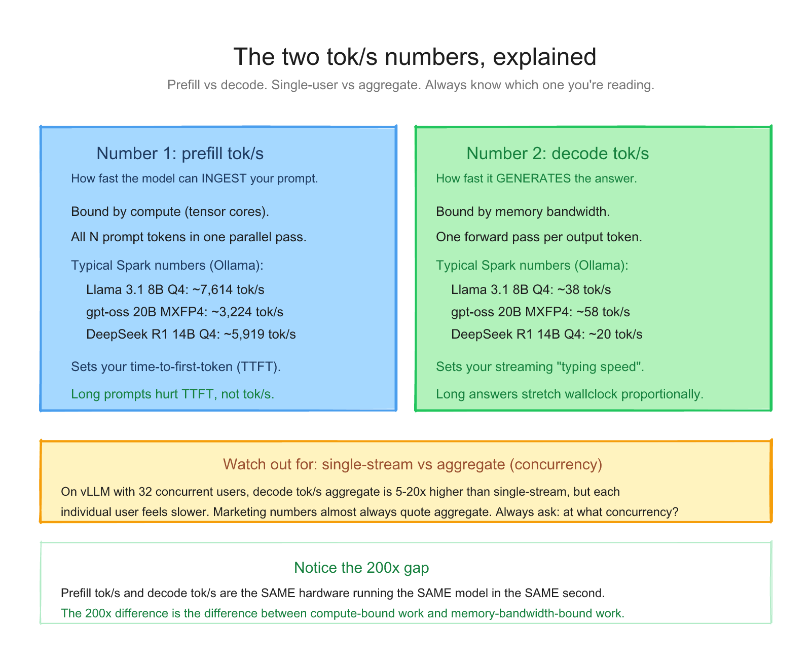
When someone says "this model runs at 50 tok/s," ask them which kind. There are two:
- Prefill tok/s (time to first token, TTFT, prompt eval rate). How fast the model can ingest your prompt. Compute-bound. High numbers, typically 1,000-10,000+ on Spark.
- Decode tok/s (output generation rate, eval rate). How fast the model can produce new tokens. Memory-bandwidth-bound. Lower numbers, typically 5-100 on Spark depending on model size and quantization.
If your workload is "long prompt, short answer" (RAG, summarization), prefill speed dominates user-perceived latency.
If your workload is "short prompt, long answer" (coding, essay generation), decode speed dominates.
If your workload is "long prompt, long answer" (agentic, complex tasks), both matter.
Ollama reports both. So does vLLM. Looking at the actual numbers Ollama published for Spark:
| Model | Prefill | Decode |
|---|---|---|
| llama3.1 8B q4_K_M | 7,614 tok/s | 38 tok/s |
| gpt-oss 20B MXFP4 | 3,224 tok/s | 58 tok/s |
| deepseek-r1 14B q4_K_M | 5,919 tok/s | 20 tok/s |
Notice the prefill numbers are ~200x bigger than the decode numbers. Same hardware, same model, in the same second. That's the difference between compute-bound and memory-bandwidth-bound work.
Putting it together: a real request trace #
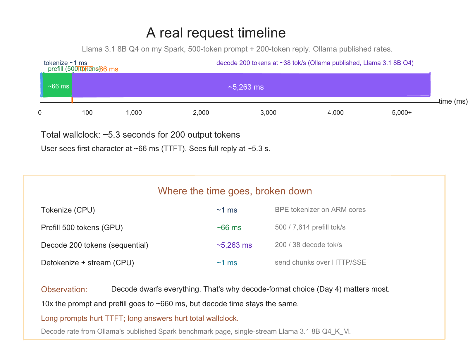
Say you send a 500-token prompt to Llama 3.1 8B Q4 on a Spark, and ask for a 200-token completion.
| Phase | Work | Time |
|---|---|---|
| Tokenize | CPU turns text into 500 integers | ~1 ms |
| Prefill | GPU reads model, computes K/V for all 500 tokens | 500 / 7614 = 66 ms |
| Decode | GPU generates 200 tokens, one at a time, reading model each time | 200 / 38 = 5.26 s |
| Detokenize | CPU turns integers back to text | ~1 ms |
| Total | ~5.3 seconds |
The user perceives "I waited 66ms for the first character, then it streamed in at ~38 tok/s." That's time-to-first-token (TTFT) = 66 ms and output rate = 38 tok/s.
Now imagine the same prompt at 16 concurrent users with vLLM batching. TTFT is roughly the same (66 ms each). For an actual measured comparison, my DGX Spark serving Qwen2.5-3B BF16 jumps from 26 tok/s single-user to 477 tok/s aggregate at c=16. For Gemma 4 31B NVFP4 the comparable jump is 6 → 92 tok/s aggregate. Serving 16 users is much closer to serving one user than your intuition expects - the exact multiplier depends on the model, but the shape always holds.
That's the local LLM serving game.
What this means for picking hardware #
If you've followed this far, you understand the hardware question.
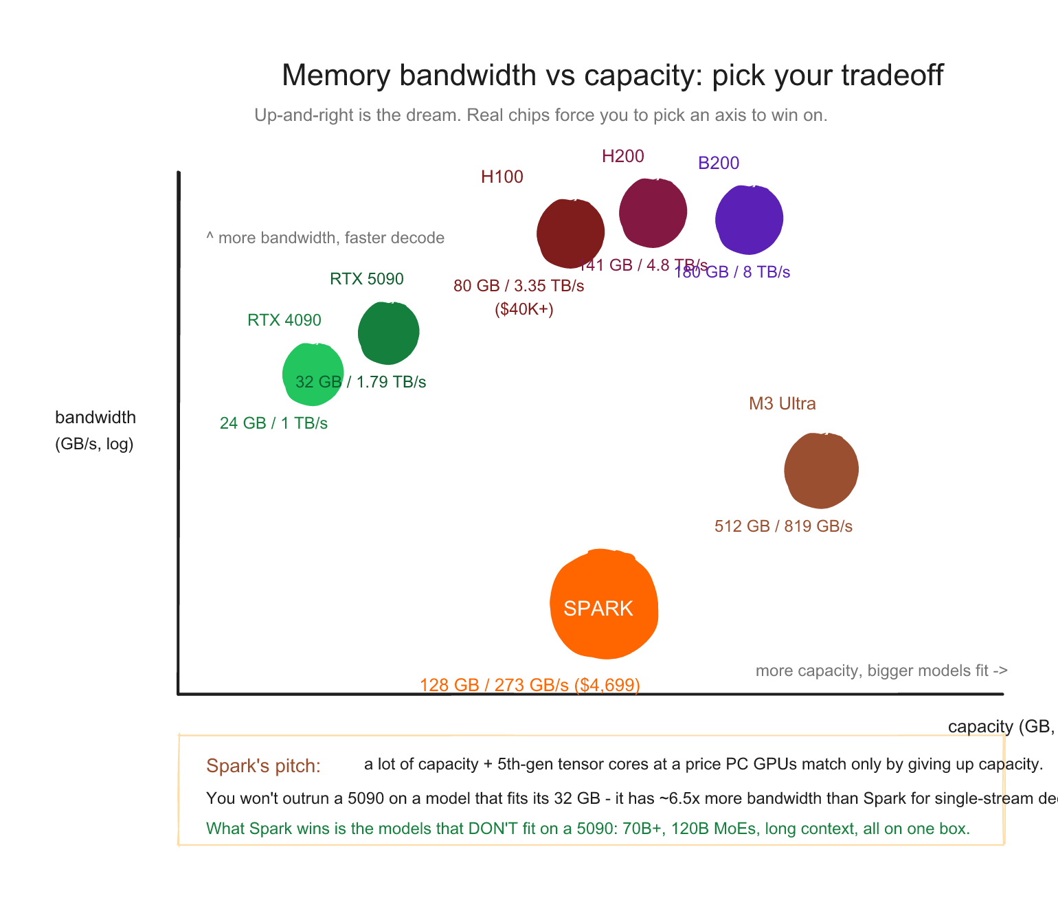
The single most important spec for LLM inference on a workstation isn't tensor core peak FLOPS. It's memory bandwidth. A single B200-class Blackwell GPU has up to about 8 TB/s of memory bandwidth, which is a different tier from Spark's 273 GB/s. An RTX 5090 with 1,792 GB/s beats a Spark on bandwidth too, but only for models that fit in its 32 GB.
The Spark's pitch: you trade some bandwidth for a lot of capacity. 128 GB at 273 GB/s lets you run 70B-class and 120B-class models that simply won't fit on a 5090. The decode is slower per user. The capacity is unmatched at this price.
We open the Spark itself in the next post. By the time we get to inference-engine selection (Day 5) and the leaderboard (Day 6), you'll have the full picture.
What's coming on Day 3 #
In the next post we look at what's actually inside the GB10 Grace Blackwell Superchip. The Grace ARM CPU, the Blackwell GPU, the C2C link between them, the unified memory architecture, the sm_121 instruction set (and why it's NOT the same as datacenter Blackwell's sm_100), the 5th-generation tensor cores that execute NVFP4 natively, and the practical implications of all of it.
You'll come out understanding why a 4-bit format you've never heard of (NVFP4) is the most important thing to know about this chip.
See you in the next post.
References for this post: Ollama: NVIDIA DGX Spark performance for the published prefill and decode numbers, vLLM documentation for batching and KV cache concepts. The concurrency sweep tables are from my own measurements on this Spark on 2026-05-21 (Gemma 4 31B IT NVFP4 + Qwen2.5-3B BF16 via vLLM at max_tokens=512). An earlier 2026-05-08 sweep had a concurrency-label drift; the 2026-05-21 values are canonical.
Saiyam is working as Head of DevRel at vCluster Labs. He is the founder of Kubesimplify, focusing on simplifying cloud-native & AI infrastructure. He is KubeCon Co-chair and has worked on many facets of Kubernetes, including machine learning platforms, scaling, multi-cloud, & managed Kubernetes services. When not coding, Saiyam contributes to the community by writing blogs and organizing local meetups for Kubernetes and CNCF. He is also a CNCF TAG OpsRes Chair & can be reached on Twitter @saiyampathak.
Get new posts in your inbox.
Spotted a typo or want to improve this post? Edit on GitHub →